In my previous project, I developed the reasoning behind Hidden Markov Models (HMM) and developed a way of determining the most likely sequence of states that resulted in an observed sequence of emissions using the Viterbi algorithm. This project will explore extensions to the Hidden Markov Model, such as the Forwards-Backwards algorithm and the Baum-Welch algorithm.
Consider a discrete time, discrete state-space Hidden Markov chain with:
- $\pi_{t}$ : the state at time t (unknown in the HMM) of n possible states
- $\pi_{t} = 1,2,\ldots,n$
- $x_{\text{t}}$: the emission at time t of m possible emissions,
- $x_{\text{t}} = 1,2,\ldots,m$
- P(0) : initial probabilities of being in the states.
- P : a nxn transition matrix of transitions between states, giving P($\pi_{t} = i\left| \pi_{t - 1} = j \right)$ for the ith row and jth column.
- E : a nxm matrix containing P($x_{\text{t}} = j\ \left| \ \pi_{t} = i \right)$ in the ith row, jth column, the emission probabilities. Note that the row sums must sum to 1.
Given a set of observed emissions, $x_{1,\ldots,\ T}$, the Viterbi algorithm gives us the most likely sequence of states, $\pi_{1,\ldots,\ T}$ that resulted in the observed emissions, given P and E.
Although this decoding algorithm is very useful, there may be other aspects of the HMM we are interested in. One such problem is, given a set of observed emissions $x_{1,\ldots,\ T}$, what is the probability of the observed emissions? This problem can be solved using the law of total probability, i.e.:
$$P\left( x_{1},\ \ldots,x_{T} \right) = \ \sum_{\mathbf{\pi}}^{}{P(x_{1},\ \ldots,x_{T}}\left| \ \mathbf{\pi} \right)P(\mathbf{\pi})\ $$where $\mathbf{\pi}$ refers to any vector of state sequences. This can be computationally intensive -- for many steps, this will involve summing over an exponentially large number of possible state sequences. Thus, an algorithmic approach will be useful to make this result practical to obtain for large T. This is a similar problem to the Viterbi algorithm, but not exactly the same. This can be solved using the forward algorithm, as described below. Note that we can also write the above as:
$$P\left( x_{1},\ \ldots,x_{T} \right) = \ \sum_{\mathbf{\pi}}^{}{P(x_{1},\ \ldots,x_{T}},\mathbf{\pi})\ $$Let's call $\alpha_{t}(\pi_{t})$ = $P\left( x_{1},\ \ldots,x_{t},\ \pi_{t} \right) = \ \sum_{\pi_{t - 1}}^{}{P(x_{1},\ \ldots,x_{T},\ \pi_{t},\pi_{t - 1})}$
It follows that our desired probability of the sequence is equal to the sum over all states of the above quantity.
$$\alpha_{t}(\pi_{t}) = \ \sum_{\mathbf{\pi}_{t - 1}}^{}{P(x_{t}|x_{1},\ \ldots,x_{t - 1},\ \pi_{t},\ \pi_{t - 1})P(\pi_{t}|x_{1},\ \ldots,x_{t - 1},\ \pi_{t - 1}})P(x_{1},\ \ldots,x_{t - 1},\ \pi_{t - 1})$$But $x_{t}$ is conditionally independent of everything but $\pi_{t},\ $and $\pi_{t}$conditionally independent on everything but $\pi_{t - 1}$. So we can write this simply as:
$$\alpha_{t}(\pi_{t}) = \ P(x_{t}|\pi_{t})\sum_{\mathbf{\pi}_{t - 1}}^{}{P(\pi_{t}|\pi_{t - 1}})P(x_{1},\ \ldots,x_{t - 1},\ \pi_{t - 1})$$$$= \ P(x_{t}|\pi_{t})\sum_{\mathbf{\pi}_{t - 1}}^{}{P(\pi_{t}|\pi_{t - 1}})\alpha_{t - 1}(\pi_{t - 1})$$It follows, then, that we can compute each $\alpha_{t}$ recursively. This will eliminate the need to look at the probability of all states. This has a computation time of $O(\text{nm}^{2})$ which is far faster than doing it for each possible sequence, which is$\ O(\text{nm}^{n})$. After computing this for each possible state at time T, we sum the probabilities to get the probability of the observed sequence. Note that $\alpha_{1}\left( \pi_{1} \right) = P(x_{1}|\pi_{1})\sum_{x_{0}}^{}{P(\pi_{1}|\pi_{0}})P(\pi_{0}) = \ \ P(x_{1}|\pi_{1})P(\pi_{1})$, where $P\left( \pi_{1} \right)$ is to be considered the initial probabilities of entering the chain, predefined by the problem.
Consider the following example of a fair and biased coin, where:
Initial probabilities are equal, .5 for fair and .5 for biased
$$\mathbf{P = \ }\begin{matrix} .9 & .1 \\ .05 & .95 \\ \end{matrix}$$$$\mathbf{E = \ }\begin{matrix} .5 & .5 \\ .25 & .75 \\ \end{matrix}$$We observe the sequence HTHHTTHH and want to determine the probability of this sequence occurring given our HMM. First,
$$\alpha_{1}\left( \pi_{1} = F \right) = \ P\left( x_{1} \middle| \pi_{1} = F \right)P\left( \pi_{1} = F \right) = \left( 0.5 \right)\left( 0.5 \right) = \ .25$$$$\alpha_{1}\left( \pi_{1} = B \right) = P\left( x_{1} \middle| \pi_{1} = B \right)P\left( \pi_{1} = B \right) = \left( 0.25 \right)\left( 0.5 \right) = \ .135$$So it follows that the probability of a head being observed, alone, is the sum of these partial probabilities, or .385. To determine the probability of the full sequence, we continue this recursively, considering the results of the function at the last time step.
We can also simplify this using matrix multiplication. If we consider $\mathbf{\alpha}_{\mathbf{t}}$ as a nx1 vector pertaining to each of the n states, we can calculate the following:
$${\mathbf{\alpha}_{\mathbf{t}}\mathbf{= \ E}}_{\mathbf{.,j}} x \mathbf{P'\alpha}_{\mathbf{t - 1}}$$Where j refers to a row vector of the jth column pertaining to the observed value at time t. This can help to simplify the calculations. Here, x refers to component-wise multiplication. I have included a user-defined function to determine this probability recursively for the problem at hand:
forwardalgor <- function(obs, trans,emissions,init){
  alphas <- list(1,init*emissions[,obs[1]])

  for(i in 2:(length(obs) + 1)){
    alphasum <- as.numeric(trans%*%alphas[[i]])
    alphas[[i + 1]] <- emissions[,obs[i-1]]*alphasum
  }
  print("Sequences:")
  print(alphas)
  print("Final Probability")
  print(sum(alphas[[length(obs)+1]]))
  return(sum(alphas[[length(obs)+1]]))
}

forwardalgor(c(1,2,1,1,2,2,1,1),rbind(c(.9,.1),c(.95,.05)),rbind(c(.5,.5),c(.25,.75)),c(.5,.5))
This gives us our result -- there is about a .2% chance of this observation being output by this particular HMM. This can be useful for numerous applications: consider if one was testing against n possible HMMs. We could then find which HMM is the more likely fit by considering
$\text{argmax}_{i}(P\left( \text{HMM}_{i} \middle| x_{1},\ \ldots,x_{T} \right))$. Bayes' Rule tells us that:
$$P\left( \text{HMM}_{i} \middle| x_{1},\ \ldots,x_{T} \right) \propto \ P\left( x_{1},\ \ldots,x_{T} \middle| \text{HMM}_{i} \right)P(\text{HMM}_{i})$$If we consider our n models as equally likely, we can then determine which model is most probable given the observations simply by considering the likelihood in the fashion calculated above. That is, $\operatorname{}\left( P\left( \text{HMM}_{i} \middle| x_{1},\ \ldots,x_{T} \right) \right) = \text{argmax}_{i}(\ P\left( x_{1},\ \ldots,x_{T} \middle| \text{HMM}_{i} \right))$. This relatively simple result and simple algorithm gives us a method of comparing and optimizing our fit. Also, since the probabilities here can become quite small, the fact that a logarithmic function is monotonically increasing means we can also compare the logarithms, in order to avoid machine zeros.
The closely related, but not exactly equivalent, Forwards-Backwards algorithm attempts to find probability of a particular state of a particular time point given all of the observations, i.e. :
$$P({\pi_{k}|x}_{1},\ \ldots,x_{T})$$$$P\left( {\pi_{k}|x}_{1},\ \ldots,x_{k,\ }x_{k + 1},\ldots,x_{T} \right) = \ \frac{P\left( x_{k + 1},\ldots,x_{T}|{\pi_{k},x}_{1},\ \ldots,x_{k} \right)P\left( {\pi_{k}|x}_{1},\ \ldots,x_{k} \right)}{P\left( x_{k + 1},\ldots,x_{T} \right)}$$$$\propto P\left( x_{k + 1},\ldots,x_{T}|\pi_{k} \right)P\left( {\pi_{k}|x}_{1},\ \ldots,x_{k} \right)$$
This is due to the fact that $x_{k + 1},\ldots,x_{T}$ is conditionally independent of $x_{1},\ \ldots,x_{k}$ given $\pi_{k}$ and that $P\left( x_{k + 1},\ldots,x_{T} \right)$ is a multiplicative constant which does not change with a selection of $\pi_{k}$. This means we can normalize this probability at each point to ensure that $\sum_{}^{}{P\left( {\pi_{k}|x}_{1},\ \ldots,x_{k,\ }x_{k + 1},\ldots,x_{T} \right) = 1}$. Notice that $P\left( {\pi_{k}|x}_{1},\ \ldots,x_{k} \right)\ \propto \ P\left( x_{1},\ \ldots,x_{k},\ \pi_{k} \right) = \ \alpha_{k}\mathbf{(}\pi_{k})$ as described earlier.
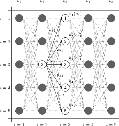
Notice that $P\left( x_{k + 1},\ldots,x_{T}|\pi_{k} \right)$ is a similar proposition, but backwards. That is, we can call $$b_{k}(\pi_{k})$$ $$= \sum_{\pi_{k + 1}}^{}{P\left( \pi_{k + 1},x_{k + 1},\ldots,x_{T}|\pi_{k} \right)}$$ $$= \sum_{\pi_{k + 1}}^{}{P\left( x_{k + 2},\ldots,x_{T}|{x_{k + 1},\pi}_{k + 1},\pi_{k} \right)P(x_{k + 1}|\pi_{k + 1},\pi_{k})P(\pi_{k + 1}|\pi_{k})}$$ $$= \sum_{\pi_{k + 1}}^{}{P\left( x_{k + 2},\ldots,x_{T}|\pi_{k + 1} \right)P(x_{k + 1}|\pi_{k + 1})P(\pi_{k + 1}|\pi_{k})}$$
This is obtained using the chain rule and the conditional independencies of the HMM. Notice now that $P\left( x_{k + 2},\ldots,x_{T}|\pi_{k + 1} \right) = \ b_{k + 1}\left( \pi_{k + 1} \right)$ and we can now see the recursive nature of this function. That is,
$$b_{k}\left( \pi_{k} \right) = \ \sum_{\pi_{k + 1}}^{}{b_{k + 1}\left( \pi_{k + 1} \right)P(x_{k + 1}|\pi_{k + 1})P(\pi_{k + 1}|\pi_{k})}$$We take $b_{T}\left( \pi_{T} \right) = 1$ for all states, as this can be considered the exit probability.
Intuitively, this means that we are considering, for some intermediate time step, the probabilities of getting there from zero and the probabilities of "back tracking" from T. This gives us the total probability of an intermediate state based on our observations.
The implementation is as follows:
Compute the forward probabilities (by the previously stated algorithm) until time step k. For each step, normalize the results so that the probabilities sum to 1. Then, compute the backward probabilities from T to k. Normalize these at each step as well. Then, multiply the two results and normalize to get the probabilities of being in each state after k time steps.
To calculate this, we may use the following formula:
$${\mathbf{b}_{\mathbf{t}}\mathbf{= \ P(E}}_{\mathbf{.,j}} x \mathbf{b}_{\mathbf{t + 1}}\mathbf{)}$$Notice that this is similar to the formula from before for the forwards portion, but the multiplications are "flipped." Thus we can implement the Forward-Backwards algorithm as follows:
bkforwardalgor <- function(obs, k, trans, emissions, init) {
    alphas <- list(1, init * emissions[, obs[1]]/sum(init * emissions[, obs[1]]))
    betas <- list(rep(1, nrow(trans)))

    for (i in 3:(k + 1)) {
        alphasum <- as.numeric(t(trans) %*% alphas[[i - 1]])
        alphas[[i]] <- emissions[, obs[i - 1]] * alphasum
        alphas[[i]] <- alphas[[i]]/sum(alphas[[i]])
    }
    for (i in 2:(length(obs) - k + 1)) {
        betasum <- emissions[, obs[length(obs) - i + 2]] * betas[[i - 1]]
        betas[[i]] <- as.numeric(trans %*% betasum)
        betas[[i]] <- betas[[i]]/sum(betas[[i]])
    }
    pointalph <- alphas[[(k + 1)]]
    pointbet <- betas[[(length(obs) - k + 1)]]

    return(list(forward = alphas, backward = betas, probstates = pointalph * pointbet/sum(pointalph *
        pointbet)))
}


bkforwardalgor(c(1, 2, 1, 1, 2, 2, 1, 1), 3, rbind(c(0.9, 0.1), c(0.95, 0.05)), rbind(c(0.5,
    0.5), c(0.25, 0.75)), c(0.5, 0.5))
So, at the third time step, we are close to 95% certain that we were in the first state (Heads), given all of the observations.
This all leads us to the Baum-Welch algorithm, which is a way of estimating parameters of a HMM given a sequence of emissions. Let $\gamma_{i}\left( t \right) = P\left( \pi_{t} \middle| \theta,x_{1},\ \ldots,x_{T} \right)$ where $\theta$ is the parameters of the distribution (the transition matrix, the emission matrix and the initial probabilities.) Note that we have already calculated this in the previous exercise using the forwards backwards algorithm.
Further, let $$\xi_{i,j}\left( t \right) = \ P\left( \pi_{t}\ ,\pi_{t + 1}\ \middle| \theta,x_{1},\ \ldots,x_{T} \right) = \frac{\alpha_{t}\left( \pi_{t} = i \right)\mathbf{P}_{\text{ij}}b_{t + 1}\left( \pi_{t + 1} = j \right)\mathbf{E}_{{j,x}_{t + 1}}}{\sum_{}^{}{\alpha_{t}\left( \pi_{t} = i \right)\mathbf{P}_{\text{ij}}b_{t + 1}\left( \pi_{t + 1} = j \right)\mathbf{E}_{{j,x}_{t + 1}}}}$$
This represents the probability of entering state i from the left, going from state i to j, exiting state j from the right, and emitting the emission at the t+1 time step from state j. All of this culminates in the joint probability of two consecutive states.
Then, using an initial set of parameters we can calculate these values and update our parameters to find a local maxima. Our updates are as follows:
Initial probabilities = $\gamma_{i}\left( 1 \right)$. This is the expected frequency spent in state i at time 1.
The new transition matrix, P', will have entries:
$$\mathbf{P'}_{\text{ij}} = \frac{\sum_{t = 1}^{T - 1}{\ \xi_{i,j}\left( t \right)}\ }{\sum_{t = 1}^{T - 1}{\gamma_{i}\left( t \right)}}$$This is the expected number of transitions from state i to j compared to the expected total number of transitions away from state i (including itself).
The new emission matrix, E', will have entries:
$\mathbf{E'}_{\text{ij}} = \frac{\sum_{t = 1}^{T}1_{x_{t} = j}\gamma_{i}\left( t \right)}{\sum_{t = 1}^{T}{\gamma_{i}\left( t \right)}}$
Where $1_{x_{t} = j}$ is an indicator function which is 1 if the emission was the jth emission and zero otherwise. This calculates the average amount of time an emission j was emitted in state i divided by the average amount of time it was in state i in general.
We then iterate this process until we are within a threshold to determine the optimal parameters for the model given only an observed sequence.
While I have not implemented this algorithm directly here, I have used the HMM package in R to determine this. Here is the output:
library(HMM)
chk <- initHMM(States = c("F","B"),Symbols = c("H","T"),startProbs = c(.5,.5),
               transProbs = rbind(c(.9,.1),c(.95,.05)), emissionProbs = rbind(c(.5,.5),c(.25,.75)))
baumWelch(chk,c("H","T","H","H","T","T","H","H"))
Here, we see that the algorithm suggests changing the transition probabilities to almost never transition when in the Biased state, and to transition more frequently when in the fair state. It also suggests that the emission probabilities be heads nearly in all cases when it is biased. This is troublesome, since we knew (by our definition) that the emissions would be fair for the fair coin and biased otherwise. Still, this generalizes the problem and allows us to attempt to fit optimal HMMs to a given set of emissions.
Using the Viterbi algorithm is known as "decoding" -- we are attempting to determine the most likely state sequence given a sequence of observed emissions. Determining the most likely state at a time step is known as "filtering" (when the step is the final step, T) or "smoothing" (for some intermediate step, k). This is what the forward-backward algorithm was used for. Attempting to determine the best fitting parameters is known as "training". This is the motivation of the Baum-Welch algorithm. Together, these three algorithms provide the basis for many applications of the HMM model.